Sparse Voxel Octrees in Haskell

It's been a long time coming (daughters birth impedes Haskell coding!), but I've finally implemented and uploaded support for Sparse Voxel Octrees in my Haskell Renderer.

It's quite an interesting algorithm to implement in something like Haskell. It's interesting because it really questions the balance of strict vs lazy evaluation in Haskell. Which is better - strict construction and strict traversal, with the platform optimisations that may bring, or lazy construction-as-you-traverse?

In an imperative language, you'd run a complete process to construct the tree, and then traverse the completed tree for each intersection query. You have to pay the total construction cost plus the traversal cost. Since you'd be constructing and storing the whole tree, you need to invest significant effort in data compression. On the other hand, the direct data representation would permit you to make a number of optimisations aimed at evaluation efficiency.

With Haskell, the lazy evaluation thunks can do some of that work for you. Instead of trying to crunch the whole tree down to be as small as possible, you may choose instead to rely on the Haskell runtime to just-in-time construct the relevant portions of it. You would only pay the cost of construction for the parts of the tree you traverse. Would this sum be lower than a strict construction and traversal?

Alternatively, In Haskell, you can still go for the strict option and implement it much as you would with C.

What's interesting is that it introduces this challenging, general question of what offers the most efficiency: A domain-specific, efficiently implemented clever algorithm, or a somewhat more generic algorithm, less specifically optimised but instead relying on lazy evaluation and the higher-order optimisations that may automatically permit?

I'm not sure what the answer is to this question right now. I suspect there is a cross over point that is very specific to the data set in question and therefore your particular application.

Code

My current Haskell SVO code is on github, in my Haskell Renderer:

https://github.com/TomHammersley/HaskellRenderer

I'm going to fix up the various remaining TODOs and then pursue a more optimised, C-like version along the lines of the various SIMD-like SVO implementations that have recently emerged.

Implementation Notes

This was ultimately quite an elegant algorithm to implement in Haskell. Much of the algorithm is built off simple geometric tests. These are quite compact and elegant to represent in a functional language like Haskell. For instance, a ray-box test is simply:

boundingBoxIntersectRay :: AABB -> Ray -> Maybe (Double, Double)
boundingBoxIntersectRay (bounds0, bounds1) (Ray rayOrg _ invRayDir rayLen)
     | tmax > tmin = Nothing
     | tmin > 0 && tmin < rayLen = Just (tmin, tmax `Prelude.min` rayLen)
     | tmax > 0 && tmax < rayLen = Just (tmax, tmax)
     | otherwise = Nothing
where
     (tmin, tmax) = foldr1 (\(a0, b0) (a1, b1) -> (a0 `Prelude.max` a1, b0 `Prelude.min` b1)) (map intercepts [vecX, vecY, vecZ])


intercepts f = let x0 = (f bounds0 - f rayOrg) * f invRayDir
                   x1 = (f bounds1 - f rayOrg) * f invRayDir
               in (x0 `Prelude.min` x1, x0 `Prelude.max` x1)

Here we simply define an operation to calculate the slab intercepts of the box, and then repeat that operation over X, Y and Z, then fold to reduce the results. We're offering a description of the algorithm to Haskell in high level primitives, permitting optimisation and reduction - as opposed to clumsily trying to indirectly tell a C++ compiler what you'd really like it to do. It's surprising how often this sort of thing proves faster in Haskell. For example, using the "any" or "all" functions has proven faster than a set of || or && clauses for me in the past. I could really imagine that a thunk-less version of Haskell, free of the irritation of considering C++ aliasing might produce some very efficient code.

The traversal code is a simple recursive traversal, with few (as yet) clever tricks. It terminates either at the leaves, at the maximum traversal depth or when the feature becomes too small when projected to screen space (though this calculation needs further elaboration). It therefore gives a simple, automatic LOD control.

And so, finally, here it is, our SVO lego-sphere:

Haskell Photon Mapper Released to Hackage

I've now uploaded my Haskell photon mapper and raytracer to hackage. It is listed as a package called "crocodile" (named after my son's current obsession with crocodiles!).

It's all working on the Cornell box. It's pretty memory hungry, and has a few self-declared things to fix (eg irradiance gradients), but it's out there to play with.

Enjoy.

Photon Mapping in Haskell

For a while I have been working on extending my Haskell raytracer to include a global illumination model. I chose to implement photon mapping, as it seemed to offer both a number of challenges, and it quite suited a functional programming approach.

Photon Tracing

One of the main challenges of implementing an algorithm like photon mapping is that it relies on a small amount of mutable state due to its monte-carlo integration. As each photon is traced through the scene, a random number is required to determine the fate of a photon for a given photon-to-material interaction. A random number generator typically requires state to iterate from one number to the next. Such state is easy to incorporate into imperative code, but it presents a challenge to the Haskell programmer.

There are two main challenges with state: management and propagation of state, and selecting what code should share a given state context. For example, in the photon mapper I could have introduced a single, global state for the random number generator. Or, I could have given each light source its own state. Or each photon. The greater scope that the state has, the greater the coupling in the code and the greater the difficulty in parallelisation.

I chose to give each photon traced its own random number generator state - and each photon had a different initial seed.

-- Realistic Image Synthesis Using Photon Mapping p60
tracePhoton :: [Photon] -> Photon -> SceneGraph -> StdGen -> (Int, Int) -> [Photon]
tracePhoton !currentPhotons (Photon !photonPower !photonPosDir) sceneGraph !rndState !(bounce, maxBounces) = 
    -- See if the photon intersects any surfaces
    case findNearestIntersection sceneGraph ray of
      Nothing -> currentPhotons
      Just (obj, t, subId) -> case photonFate of
                                -- Diffuse reflection. Here, we store the photon that got reflected, and trace a new photon - but only if it's bright enough to be worthwhile
                                DiffuseReflect -> if Colour.magnitude newPhotonPower > brightnessEpsilon && (bounce + 1) <= maxBounces
                                                  then tracePhoton (storedPhoton : currentPhotons) reflectedPhoton sceneGraph rndState'' (bounce + 1, maxBounces)
                                                  else storedPhoton : currentPhotons
                                    where
                                      !reflectedPhoton = Photon newPhotonPower (surfacePos, reflectedDir)
                                      !(reflectedDir, rndState'') = diffuseReflectionDirection rndState' tanSpace


                                -- Specular reflection. Here, we reflect the photon in the fashion that the surface would reflect towards the viewer and
                                -- aim to absorb it somewhere else in the photon map
                                SpecularReflect -> if Colour.magnitude newPhotonPower > brightnessEpsilon && (bounce + 1) <= maxBounces
                                                   then tracePhoton currentPhotons reflectedPhoton sceneGraph rndState' (bounce + 1, maxBounces)
                                                   else currentPhotons
                                    where
                                      !reflectedPhoton = Photon newPhotonPower (surfacePos, reflectedDir)
                                      !reflectedDir = Vector.negate (snd photonPosDir) `reflect` normal


                                -- Absorb. The photon simply gets absorbed into the map
                                Absorb -> storedPhoton : currentPhotons
          where
            !(photonFate, rndState') = runState (choosePhotonFate coefficients) rndState
            !coefficients = russianRouletteCoefficients (material obj)
            !newPhotonPower = computeNewPhotonPower photonFate coefficients photonPower (material obj)
            !tanSpace = primitiveTangentSpace (primitive obj) subId hitPosition obj
            !normal = thr tanSpace
            !hitPosition = pointAlongRay ray t
            !surfacePos = hitPosition + (normal Vector.<*> surfaceEpsilon)
            !brightnessEpsilon = 0.1
            !storedPhoton = Photon photonPower (surfacePos, snd photonPosDir)
    where
      !ray = rayWithPosDir photonPosDir 10000

KD-Tree Construction

The resulting list of photons is inserted into a KD tree in order to efficiently locate the set of photons near to a point in space. This is a simple recursive operation:

buildKDTree :: [Photon] -> PhotonMapTree
buildKDTree photons
    | length photons == 1 = PhotonMapLeaf (head photons)
    | length photons >= 2 = let (boxMin, boxMax) = photonsBoundingBox photons
                                !axis = largestAxis (boxMax - boxMin)
                                !photonsMedian = foldr ((+) . fst . posDir) zeroVector photons Vector. fromIntegral (length photons)
                                !value = component photonsMedian axis
                                photonsGT = Prelude.filter (\x -> component ((fst . posDir) x) axis > value) photons
                                photonsLE = Prelude.filter (\x -> component ((fst . posDir) x) axis <= value) photons
                            in if length photonsGT > 0 && length photonsLE > 0
                               then PhotonMapNode axis value (buildKDTree photonsGT) (buildKDTree photonsLE)
                               else let (photons0', photons1') = trace "Using degenerate case" $ degenerateSplitList photons in PhotonMapNode axis value (buildKDTree photons0') (buildKDTree photons1')
    | otherwise = error ("Invalid case, length of array is " ++ show (length photons) ++ "\n")

KD-Tree Query

The photon mapping algorithm uses an interesting combination of a kd tree and max-heap to locate only the closest N photons to a point. The max-heap is sorted on the squared distance to a photon. This means the most distant photons are stored towards the top of the max-heap, making them easy to discard.

Traversal of the tree commences with a point of interest and a radius. Any photons found within that radius are added to the max-heap. If the max-heap exceeds its specified size then excess, distant photons are dropped from the top of the heap. Since the max-heap stores the most distant photon at the top of the heap, it is easy to monitor the current-furthest photon and tighten our search radius during traversal.


-- Use a max heap to make it easy to eliminate distant photons
data GatheredPhoton = GatheredPhoton Float Photon deriving (Show)
type PhotonHeap = MaxHeap GatheredPhoton


instance Ord GatheredPhoton where
    compare (GatheredPhoton dist1 _) (GatheredPhoton dist2 _)
        | dist1 == dist2 = EQ
        | dist1 <= dist2 = LT
        | otherwise = GT


instance Eq GatheredPhoton where
    (GatheredPhoton dist1 _) == (GatheredPhoton dist2 _) = dist1 == dist2

minimalSearchRadius !rSq !photonHeap = case viewHead photonHeap of
                                         Nothing -> rSq
                                         Just (GatheredPhoton dSq _) -> Prelude.min rSq dSq


-- Gather photons for irradiance computations
-- Algorithm adapted from Realistic Image Synthesis Using Photon Mapping p73
gatherPhotons :: PhotonMapTree -> Position -> Float -> PhotonHeap -> Int -> PhotonHeap
gatherPhotons (PhotonMapNode !axis !value gtChild leChild) !pos !rSq !photonHeap !maxPhotons
    -- In this case, the split plane bisects the search sphere - search both halves of tree
    | (value - posComponent) ** 2 <= rSq = let heap1 = gatherPhotons gtChild pos rSq' photonHeap maxPhotons
                                               rSq'' = minimalSearchRadius rSq' heap1
                                               heap2 = gatherPhotons leChild pos rSq'' photonHeap maxPhotons
                                               newHeap = union heap1 heap2
                                           in Data.Heap.drop (size newHeap - maxPhotons) newHeap


    -- One side of the tree...
    | posComponent > value = gatherPhotons gtChild pos rSq' photonHeap maxPhotons


    -- ... or the other
    | posComponent <= value = gatherPhotons leChild pos rSq' photonHeap maxPhotons


    -- Prolapse
    | otherwise = error "gatherPhotons: unexplained/unexpected case here"
    where
      !posComponent = component pos axis
      !rSq' = minimalSearchRadius rSq photonHeap -- Refine search radius as we go down tree to search no further than closest allowed photon
gatherPhotons (PhotonMapLeaf !p) !pos !rSq !photonHeap !maxPhotons
    | distSq < rSq = let newHeap = insert (GatheredPhoton distSq p) photonHeap
                     in Data.Heap.drop (size newHeap - maxPhotons) newHeap -- Discard any excess photons - we get rid of the furthest ones
    | otherwise = photonHeap
    where !distSq = pos `distanceSq` (fst . posDir) p

Parallelisation

The photon tracing stage is trivially easy to parallelise, provided that you have carefully treated the shared state required by the random number generator. Since I have provided each traced photon with it's own state, which is uniquely initialised, all photons are data independent and therefore easy to trace in parallel.

I have not yet parallelised the photon gathering stage, due to some issues with the current implementation's efficiency. Two options present themselves for parallelisation. The first is to parallelise the traversal of high-level sub-branches of the KD tree. This naive approach would yield some speedup, but the work of each thread is likely to be highly unbalanced.

Speculatively, a work-stealing queue type approach may help here. The high-level nodes to be traversed could be initially inserted into a queue. When a worker thread pulls data, it could compare how many nodes remain to be traversed against the total number of workers. If the ratio of nodes:workers becomes very low, nodes could be repeatedly removed from the queue and replaced with their child nodes, until the ratio becomes favourable. This would populate the queue with a fairly heterogenous mixture of large and small amounts of work to be done, which would help fill up and balance processor time across the threads.

Results

Here is the current output image, with all options cranked up:

The code requires refinement and tuning to eliminate the bias, improve the colour bleeding and fix a few minor artefacts.

The photon mapper is currently very slow. It can take hours on my MacBook Pro to trace a scene containing 100,000 photons, and that is a very small number of photons.

Most of the time is spent in the gathering phase. The current implementation is very space intensive and requires further serious attention. The photon emission and tracing step, however, is extremely quick, requiring only a few seconds to trace 100,000 photons.

Code

Full source code is available on github:

https://github.com/TomHammersley/HaskellRenderer

Future Work

I am now working to improve the efficiency of the gathering phase which will improve efficiency and development speed. I am also implementing an irradiance cache to further optimise execution speed. Clearly various minor bugs also need addressing.

References

Further implementation details can be found primarily in Henrik Wann Jensen's photon mapping book, supplemented by various SIGGRAPH course materials.

Haskell Renderer Source Code on Github

Just a quick note to let anyone interested that the source code to my work-in-progress Haskell raytracer and photon mapper is now available at:

https://github.com/TomHammersley/HaskellRenderer

I'm currently mid way through debugging and optimising the photon map solution. It works, though it takes 10 minutes or so on my MacBook Pro.

When run it will output the following image:

To build the program you just need the latest Haskell Platform and the bmp package from cabal.

I'm still a beginner at Haskell so some of the code may not represent the most idiomatic or best practice Haskell. If anyone has any advice, comments or constructive criticism, I'm keen to hear it at tomhammersley@gmail.com.

(I plan to make the package Cabal compatible soon).

Cheers.

Ray-Triangle Intersection in Haskell

Recently, I've been experimenting with different ray-triangle intersection algorithms. There are many alternatives out there, and many more optimisations and special cases, but I was looking for an version that ran quickly, and "suited" functional programming.

I settled on the half-planes solution. This algorithm defines a plane at each edge of the triangle by crossing the triangle's normal and the edge direction. To check if a triangle is inside the triangle, you simply check to see if a point (on the plane of the triangle) is on the same side of all of those planes.

This costs a little extra storage space, but it's a very fast test.

So. How does the code pan out? Well, pointInsideTriangle is simple enough:



distanceToPlane :: Shape -> Vector -> Float
distanceToPlane (Plane !norm !dist) !pos = pos `dot3` norm + dist
distanceToPlane _ _ = undefined



pointInsideTriangle :: Triangle -> Position -> Bool
pointInsideTriangle !tri !point = foldr (&&) True $ map (\pln -> (distanceToPlane pln point) >= 0) (halfPlanes tri)

This is best read right-to-left. The map applies a lambda function to each of the half planes. This function simply returns a bool, telling us if a point is on the correct side of a triangle. This yields a list of bools. We need to turn that into a single result; this is done using a fold to reduce many values to a single Bool. I've deliberately used a right-fold so that the fold lazily consumes only the necessary parts of the list. It can early-out.

So there we have it. One line of Haskell (with a couple of helper functions) to do the test.

The rest of the Haskell code for a ray-triangle intersection is pretty straightforward:

intersectRayTriangle :: Ray -> Object -> Triangle -> Bool -> Maybe (Float, Triangle)

intersectRayTriangle !ray !obj !triangle !doubleSided

    | doubleSided == False && (direction ray) `dot3` (normal $ plane triangle) > 0 = Nothing

    | otherwise = case shapeClosestIntersect (plane triangle) ray obj of

                    Nothing -> Nothing

                    Just (dist', _) -> if pointInsideTriangle triangle (pointAlongRay ray dist')

                                       then Just (dist', triangle)

                                       else Nothing

Here we have a simple guard condition to permit backface culling. If the triangle is not double-sided, we do a backface culling test and possibly reject it. If not, we fall through to the default case and intersect the ray against the plane, and then test that intersection point for containment in the triangle.

Intersecting against a list is an interesting case. A simple version would just map against the list, and then attempt to find the closest intersection out of the resulting list. However, if we use tail recursion, we can add a parameter to hold our current "state" and therefore maintain a current-closest intersection. This eliminates a second search-the-list step, and also permits an early-reject optimisation:

intersectRayTriangleList :: [Triangle] -> Int -> Maybe (Float, Int) -> Ray -> Object -> Maybe (Float, Int)

intersectRayTriangleList !(x:xs) !index !currentResult !currentRay !obj = intersectRayTriangleList xs (index + 1) newResult newRay obj

    where

      (newRay, newResult) = case intersectRayTriangle currentRay obj x False of

                              Nothing -> (currentRay, currentResult)

                              Just (dist, _) -> (shortenRay currentRay dist, Just (dist, index))

intersectRayTriangleList [] _ !currentResult _ _ = currentResult

The pattern of "searching a list of x and return the closest" occurs frequently in raytracing. This is a potential candidate to be factored out into a re-usable function, or possibly even a monad.

The resulting code is also quite efficient. I'm now running at less than a minute for my test scene of the Cornell Box with 8x8 distributed raytracing. This is 30% quicker than my previously Möller-Trumbore ray-triangle intersection test.

How to Parallelise A Haskell Raytracer

One of the big attractions of functional languages is that they're theoretically very easily to parallelise as they have no problematic side-effects You only describe how to perform a calculation, and never touch on the details of moving data around the machine. The run-time is then free to process data, given your functional expressions, in parallel.

I've been experimenting with Haskell's basic parallelism primitives, par, and pseq. These primitives trigger ("spark") evaluation of expressions in parallel - but only if the runtime deems it necessary.

After many failed or mildly successful experiments, I've finally managed to get a speedup. In short, I stopped trying to reinvent the wheel myself. I simply used parListChunk:


rayTraceImage :: Camera -> Int -> Int -> SceneGraph -> [Light] -> [Colour]
rayTraceImage camera renderWidth renderHeight sceneGraph lights = map (clamp . tracePixel eyePosition sceneGraph lights) rayDirections `using` parListChunk 256 rseq
    where !rayDirections = [makeRayDirection renderWidth renderHeight camera (x, y) | y <- [0..(renderHeight - 1)], x <- [0..(renderWidth - 1)]]
          !eyePosition = Camera.position camera

Here, we break the list of rays to be traced into data parallel chunks of 256, each free to be evaluated by a different thread. Each of these chunks is processed using map. Map applies the raytracing function to convert a ray direction into a colour, and we clamp the result.

And that's it.

Running it on two threads on my dual-core MacBook Pro halves the execution time.

What's nice is that the core 'map' expression is separated from the details of parallelisation. We've separated the concepts of raytracing and its parallel decomposition into two separate concerns. We are therefore free to vary either without intertwining their concerns.

Not a critical section, lock-free queue or atomic operation in sight!

Clearly, the nature of the functional approach surrenders a lot of low-level implementation details to your platform's runtime. However, it is more frequently the case that when you require such low-level intervention, you are working around deficiencies in your run-time platform, rather than dealing with fundamental algorithm details. Parallelising many algorithms follows established patterns.

It is also worth noting that the raytracer code is currently pretty straightforward code. I've not implemented any particular tricky optimisations, and certainly none of the ideas in work such as Ingo Wald's parallel raytracing PhD thesis. Not yet, anyway...

Laziness vs Strictness in Haskell

I've just taken over a minute of execution time off my raytracer.

One of Haskell's biggest language features is the lazy evaluation system. By default, Haskell evaluates nearly all expressions lazily, as needed. This is one of the features that drew me to Haskell, and indeed it seems a reasonably apt way of writing a raytracer. Raytracing often consists of selectively traversing different parts of large databases for different parts of the scene. Many acceleration schemes involve simple mechanisms to lazily evaluate results.

Laziness, however, does pose an overhead. Haskell introduces a "thunk" for every lazy expression. A thunk describes how to calculate a deferred expression when required. For some expressions, a thunk is a potential time saver: you can defer work until needed, calculate the required value, then re-use it. For other things, such as simple arithmetic operations like vector addition, a thunk is an overhead often comparable to the original operation.

Haskell offers a couple of ways to avoid thunks and therefore lazy evalation. The main two I use are the BangPatterns extension to explicitly mark something as strictly (ie, non-lazily) evaluated, and seq.

The BangPatterns extension allows you to mark expressions that you want to be explicitly evaluated with a !. So, for a Vector, you would write Vector !Float !Float !Float !Float. This way, you force anything you assign to a vector to be strictly evaluated and stored in the vector.

Seq is used to strictly force the evaluation of a function. Seq has the signature of a -> b -> a. It therefore takes two parameters, and returns the second.

An interesting example of where lazy evaluation proven to be an overheard, rather than a win was my light accumulation function. Given a point in space to be shaded, this accumulates the contribution of every light source. Now, the inputs to this function are going to be different every time this function is called as every ray intersection is going to be unique. Thunks will therefore present an additional overhead.

I rewrote my function to use seq. I use seq to strictly evaluate the application of this function, then process the remainder of the list:


accumulateLight :: [Light] -> Colour -> SceneGraph -> Vector -> Vector -> Material -> Vector -> Colour
accumulateLight (x:xs) acc sceneGraph shadePos normal objMaterial viewDirection = let result = acc + (applyLight sceneGraph shadePos normal objMaterial viewDirection x)
                                                                                  in seq result (accumulateLight xs result sceneGraph shadePos normal objMaterial viewDirection)
accumulateLight [] acc _ _ _ _ _ = acc

This change alone saved over a minute of execution time! Since a raytracer generally consists of many similar kinds of loops, I am now searching for wider application of this technique. It's a very difficult call to make with a limited data set. Some functions may be faster if strictly evaluated with a small dataset, but may perform better if evaluated lazily with a larger dataset.

Profiling will guide me.

Sphere Tree Construction and Traversal in Haskell

Finally. I've finally finished writing and debugging my sphere tree construction code in Haskell.

It should have been so easy. Tree structures are very easily recursively defined which is ideal for functional languages like Haskell. Take your data, split it up, and build the children by recursion. Simple. Only it was anything but...

The logic of the task was simple enough. The main problem was debugging. This is the sort of task that is prone to simple mistakes that cause time-consuming debugging problems. When working in an imperative language, you can easily put down a breakpoint and inspect your data, or if you recur too much the stack blows up, or you can step through your code and see why you're getting stuck in loops. These strategies don't map well to Haskell.

What does work in Haskell is to start small, build up gradually and constantly verify your results. You end up with a development cycle that is fundamentally very similar to test driven development. You want to prove your code one little function at a time by feeding it controlled inputs and inspecting the outputs. In Haskell, your primary debugger is your brain - you need to think very carefully through your code and how your express your algorithms. Functional languages reduce the scope of creating simple bugs due to side effects, and Haskell in particular eliminates a lot of plumbing and housekeeping code. What's left is purely your algorithm - inspect it carefully, that is where your problem lies.

Bounding Volume Hierarchies

I considered a few approaches for my bounding volume hierarchy, and for now, I've settled on a fairly generic implementation of bounding volume hierarchies that currently is configured as a sphere tree.

Each tree node can optionally (Maybe) hold an object. Each node has a sphere, but that could later be generalised. The children are defined as a list, allowing me to switch using a quadtree, kdtree or octree type approach.

(Note: The code below is best copied and viewed in a real text editor. Also, I am not yet a Haskell expert, and there may be many superior ways to achieve these results. My purpose in writing is to share my experiences as a learner with other learners.)


data SphereTreeNode = SphereTreeNode { object :: Maybe Object, children :: [SphereTreeNode], boundingRadius :: Float, boundingCentre :: Vector } deriving (Show, Read)



Sphere Tree Construction

The tree itself is constructed using a fairly simple piece of Haskell:


-- Build up a sphere tree
buildSphereTree :: ([Object] -> [[Object]]) -> [Object] -> SphereTreeNode
buildSphereTree _ (obj : []) = SphereTreeNode (Just obj) [] nodeRadius nodeCentre
    where
      nodeCentre = calculateMeanPosition (obj:[])
      nodeRadius = calculateBoundingRadius (obj:[]) nodeCentre
buildSphereTree builder (obj:objs)
    | length (obj:objs) == 1 = error "Should have been handled by a different pattern"
    | length (obj:objs) == 0 = error "Should not have zero objects"
    | otherwise = SphereTreeNode Nothing nodeChildren nodeRadius nodeCentre
    where
      nodeCentre = calculateMeanPosition (obj:objs)
      nodeRadius = calculateBoundingRadius (obj:objs) nodeCentre
      nodeChildren = map (buildSphereTree builder) (builder (obj:objs))
buildSphereTree _ [] = error "Should not hit this pattern for buildSphereTree" 

-- Find the mean of a collection of objects

calculateMeanPosition' :: [Object] -> Vector -> Vector

calculateMeanPosition' (obj : objects) acc = calculateMeanPosition' objects acc + (getCentre obj)

calculateMeanPosition' [] acc = acc

calculateMeanPosition :: [Object] -> Vector

calculateMeanPosition objects = setWTo1 ((calculateMeanPosition' objects zeroVector) fromIntegral (length objects))

-- Find the overall bounding radius of a list of objects

calculateBoundingRadius :: [Object] -> Vector -> Float

calculateBoundingRadius objs centre = foldr Prelude.max 0 (map (\obj -> shapeBoundingRadius (shape obj) (transform obj) centre) objs)

This object simply recursively builds a tree until it encounters an object list of size 1. 

I've deliberately exercised a couple of Haskell idioms here. I've used another tail-recursive loop to calculate the mean centre of the objects, and a map/fold pair to calculate the sphere's bounding radius.

The most interesting part is the first parameter to buildSphereTree. I pass in a function of type ([Object] -> [[Object]]). This function is responsible for dividing the object list into a number of lists, each of which is the object list used to build a new child node. This trick allows me to abstract out the specific algorithm for building the tree into a user-supplied function.

In my current code, I'm using a simple KD-type approach:

-- Generate a plane to split the objects along

makeSplittingPlane :: AABB -> (Vector, Float)

makeSplittingPlane (boxMin, boxMax) = case largestAxis (boxMax - boxMin) of

                                        0 -> (xaxis, -(vecX midPoint))

                                        1 -> (yaxis, -(vecY midPoint))

                                        2 -> (zaxis, -(vecZ midPoint))

                                        _ -> error "Undefined value"

    where

      midPoint = (boxMin + boxMax) <*> 0.5

-- Make children using a kd tree

generateSceneGraphUsingKDTree :: [Object] -> [[Object]]

generateSceneGraphUsingKDTree objs = leftObjects : rightObjects : []

    where

      objBox = objectListBoundingBox objs

      (planeNormal, planeDist) = makeSplittingPlane objBox

      (leftObjects, rightObjects) = partition (\obj -> planeDist + (dot3 planeNormal $ getCentre obj) > 0) objs

We simply make a splitting plane and split the list of objects according to what side of the plane their centre lies: [[Object], [Object]].

I could easily replace this function with an alternative strategy. Or even, make a function that returns a function based on the characteristics of the presented list...

Bounding Volume Hierarchy Intersection

Now this is the real meat of the implementation. The function again takes the form of a tail-recursive loop. The code is essentially similar to implementing a recursive function using a software stack in C. The tail recursion is used to make a simple loop-type recursion rather than a true state-accumulation call-type recursion.

The code is somewhat complex as several optimisations have been added.

The code is passed a list of nodes to process. We process the first node in the list, and recur with the remainder of the list - and possibly, some newly added nodes. The code seeks to find and maintain the closest-intersecting object.

The code constructs a tuple of three values - a result for this object, a list of additional nodes to process and a ray. If an object or bounding volume is hit, this tuples holds new values. If no intersection is found, we simply continue with the existing state passed into the function.

The code first considers whether the given node has any children; if it has none, it only makes sense to test the object that the node should hold. We report an error if the node has no object (a node without children or objects is useless!).

If the node does have children, it holds a subtree we wish to accept or reject. We first test the bounding volume. If this is rejected, we simply retain the current results of the loop with no additional nodes to process. If the bounding volume is intersected, then we will at least recur to the children nodes. If the node contains an object and it is intersected, we update our current intersection results and shorten our ray.

Finally, we pattern match the empty array case to simply return the current results.

Here is the code:

intersectSphereTree :: [SphereTreeNode] -> Ray -> Maybe (Object, Float, Int) -> Maybe (Object, Float, Int)

intersectSphereTree (node:nodes) ray currentHit = intersectSphereTree (newNodeList ++ nodes) newRay thisResult

    where

      -- Intersect the ray with the bounding volume of this node

      (thisResult, newNodeList, newRay) = case children node of

                                            -- If the node has no children, don't bother with it's bounding volume and just check the object (if it has one)

                                            [] -> case object node of

                                                             Nothing -> error "A node with no children should hold an object"

                                                             Just obj -> case shapeIntersect (shape obj) ray (transform obj) of

                                                                           -- Didn't hit the object. Retain the current hit, and continue with remaining nodes on the list

                                                                           Nothing -> (currentHit, [], ray)

                                                                           -- We did hit this object. Update the intersection, and continue with remaining nodes on the list

                                                                           Just (objHitDistance, objHitId) -> (Just (obj, objHitDistance, objHitId), [], shortenRay ray objHitDistance)

                                            -- We have children. In this case it makes sense to test our bounding volume

                                            nodeChildren -> case shapeIntersect (Sphere (boundingRadius node)) ray (translationMatrix' (boundingCentre node)) of -- (make a sphere centred at the object's transform matrix with given radius)

                                                              -- If we do not find an intersection, we do not update the results and we offer no further nodes to be traversed, thus skipping this subtree

                                                              Nothing -> (currentHit, [], ray)

                                                              -- If we do find an intersection against the bounding volume, then we try again against the actual object (if present)

                                                              Just (_, _) -> case object node of

                                                                               Nothing -> (currentHit, nodeChildren, ray) -- No object; just pass to the children

                                                                               Just obj -> case shapeIntersect (shape obj) ray (transform obj) of

                                                                                             -- Didn't hit the object. Retain the current hit, but offer up the children of the node as we hit the bounding volume

                                                                                             Nothing -> (currentHit, nodeChildren, ray)

                                                                                             -- We did hit this object. Update the intersection, and continue with the bounding volume's children

                                                                                             Just (objHitDistance, objHitId) -> (Just (obj, objHitDistance, objHitId), nodeChildren, shortenRay ray objHitDistance)

intersectSphereTree [] _ currentHit = currentHit

The striking thing about this code is that it steadily marches to the right of the screen, with each indentation being a new test of success or failure. Ideally, this code could be rewritten as a monad.

What About Infinite Objects?

They're simply "filter"ed out at the time of the sphere tree construction, and added to a separate list. It makes little sense to include an infinite object into any bounding volume hierarchy.

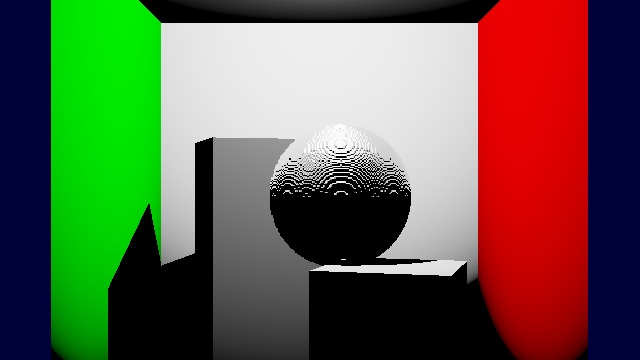
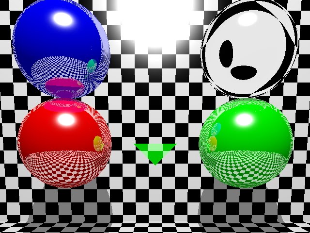
Results

The code continues to render my test scene as expected. Disappointingly, it is currently a little slower; however, this is not due to the scene graph code. I have recently rewritten my vector classes to be instances of the Num typeclass, so that I can simply write a + b, rather than coining new operators such as a <+> b. I haven't yet fully optimised my new code.

Other Observations

As I get further into Haskell, I'm finding myself increasingly thinking in terms of Lambda calculus. I no longer find myself thinking of what iterative steps I need to do to complete an operation, rather I find myself thinking in terms of the transformations of the underlying data and accompanying functions.

I find this new perspective very helpful when returning to other languages. It gives you a somewhat stream-processing-like perspective and thought process when facing standard C++ code.

What's Next?

The main focus now is to diagnose, understand and resolve the issues with my new typeclass-based fundamental data types such as Vector and Colour. I want to get it below the ~70 seconds it was previously taking. Following that, it is now time to build a parser and load some standard test scenes that will allow me to develop and optimise the ray tracer further.

A worked Haskell example

I thought it might be interesting to do a worked example of some work-in-progress Haskell to discuss what I like about it.

The case in question is the code that traverses the scene graph and intersects a ray.

Now, I'm putting the ultimate efficiency and DOD type concerns aside for a moment. I grant you there may be more efficient/better ways of doing this, it's just for discussion purposes.

Disclaimer: I am not (yet) a Haskell expert. There are probably better ways of doing this or writing it in Haskell. I write for the reasons of discussing what I've learnt about trying to write a practical application in Haskell. If there are better ways of doing it, I'd love to know, as I'm still learning.

So, first up, the code:



intersectSceneGraph' :: [SceneGraphNode] -> Ray -> Maybe (Object, Position, Int) -> Maybe (Object, Position, Int)
intersectSceneGraph' (node:nodes) ray currentHit = intersectSceneGraph' (newNodeList ++ nodes) ray thisResult
    where
      (thisResult, newNodeList) = case shapeIntersect (Sphere $ boundingRadius node) ray (transform (object node)) of
                                    Nothing -> (currentHit, [])
                                    Just (_, _) -> case shapeIntersect nodeObjectShape ray nodeObjectTransform of
                                                                   Nothing -> (currentHit, children node)
                                                                   Just (objHitDistance, objHitId) -> (Just (object node, pointAlongRay ray objHitDistance, objHitId), children node)
                                                                 where
                                                                   nodeObjectShape = shape $ object node
                                                                   nodeObjectTransform = transform $ object node
intersectSceneGraph' [] _ currentHit = currentHit


intersectSceneGraph :: SceneGraphNode -> Ray -> Maybe (Object, Position, Int)
intersectSceneGraph node ray = intersectSceneGraph' (node : []) ray Nothing

(If the code does not display clearer in your browser, cut and paste to a text editor)

This function is split into two parts. intersectSceneGraph is essentially a front end, a wrapper for intersectSceneGraph'. intersectSceneGraph' traverses a list of scene graph nodes, tests the ray against the bounding volume, and if it intersets it, it then intersects against the contained object and recurs to the children.

So, how does it traverse a tree?

The Haskell code is very similar to C code that traverses a tree using a software stack.

The operation is defined in a tail recursive fashion. I process one element of the list, and then recur to the remainder of the list. If the node in question is a new closest hit, this gets passed through to the next recursion as the new current state. If the bounding volume is intersected, then I add the children of the node to the list. If it is not intersected, I add nothing, an empty list.

This business of passing through state seems a little odd. Why would one instance of a function pass its internal state to another? This is a Haskell idiom. By passing the state from one call to another, as an "accumulator" parameter, it allows the compiler to eliminate any intermediate state on the stack and implement the recursion as a goto loop.

And all of this is lazily evaluated.

In pseudo-C, the code might look something like this:

closestHit = null;

while((topOfStack = stack.pop()) != NULL)
{

    if(intersect(ray, topOfStack->bounding volume))

    {

        if(intersect(ray, topOfStack->object))

        {

            closestHit = this one

        }

        push(stack, topOfStack->children);

    }
}

I think this shows the elegance of Haskell. Think of what is not there. There are no braces to explain scope to the compiler: you just indent it. There are no incidental variables describing the state of loop variables and so on. The compiler automatically pattern matches and dispatches to appropriate special cases instead. No pointer walks. No null checks. No explicit shuffling of data from A to B. You have a closer, more direct description of your algorithm, and the compiler fills in the gubbins.

Of course, there is a cost to all of this. By sacrificing that lower-level control, you lose out on the ultimate optimisability of the code. Still, the objective here is to find the best way to learn and use Haskell, rather than write the ultimate real-time raytracer in SIMD assembly! :-)

Depth of Field

So, I've now got depth of field working!

It was pretty straightforward. I just used a list comprehension to generate a list of points to jitter the rays with, and then it took a lot of fiddling to get the focusing working correctly.

I've also done various refactorings to my code.

All in all, it added roughly an extra 15-20 lines of code to the tracer. And that's without writing Perl-style gibberish.

Predictably enough, though, the tracer is now running much slower - about a minute for this image on my 2008 MBP. So, the next job will be learning how to optimise code in Haskell, and throwing some threading (back) in there.

Pet Project Resurrected

So, about 14 months or so ago, I spent a few weeks learning Haskell over Christmas. Then, I had to start work in earnest on my MSc final-year project, so the Haskell hacking went on the back burner.

Now that I'm in my last few weeks of the MSc, I've picked up Haskell again. Last time around I'd knocked myself up a basic little raytracer. I'm now starting up that project again. I want to work on some off-line rendering techniques for a change of pace from the day job.

So far, I've got the basics: reflection, refraction, shadows, materials and shaders (100% Haskell including shaders):

So what's next? I reckon:

* Distributed ray tracing
* Anti-aliasing
* More light types and lighting model types

That should be a good set of features to work on whilst I get my Haskell back up to speed. Once I'm back up to speed, I can start to look at meatier tasks like an asset pipeline or spatial partitioning.

I did have it running in parallel last time round, but that's all changed in Haskell in the last year or so, so I'll have to revisit that.